Steering Control Simple
Steering Control of Autonomous Vehicles in Obstacle Avoidance Maneuvers.
Contents
Vehicle model
Nonlinear model
State vector
\[ {\bf x} = \left[ \begin{array}{c} {\rm x}_1 \\ {\rm x}_2 \\ {\rm x}_3 \\ {\rm x}_4 \\ {\rm x}_5 \\ {\rm x}_6 \end{array} \right] = \left[ \begin{array}{c} x \\ y \\ \psi \\ v_{\rm T} \\ \alpha_{\rm T} \\ \dot{\psi} \end{array} \right] \]
State equations
\[ \dot{{\rm x}}_1 = {\rm x}_4 \cos \left( {\rm x}_3 + {\rm x}_5 \right) \]
\[ \dot{{\rm x}}_2 = {\rm x}_4 \sin \left( {\rm x}_3 + {\rm x}_5 \right) \]
\[ \dot{{\rm x}}_3 = {\rm x}_6 \]
\[ \dot{{\rm x}}_4 = \frac{F_{y,{\rm F}} \sin \left( {\rm x}_5 - \delta \right) + F_{y,{\rm R}} \sin {\rm x}_5}{m_{T}} \]
\[ \dot{{\rm x}}_5 = \frac{F_{y,{\rm F}} \cos \left( {\rm x}_5 - \delta \right) + F_{y,{\rm R}} \cos \alpha_{\rm T} - m_{T} {\rm x}_4 {\rm x}_6}{m_{T} {\rm x}_4} \]
\[ \dot{{\rm x}}_6 = \frac{F_{y,{\rm F}} a \cos \delta - F_{y,{\rm R}} b}{I_{T}} \]
Slip angles
\[ \alpha_{\rm F} = \arctan \left( \frac{v_{\rm T} \sin \alpha_{\rm T} + a \dot{\psi}}{ v_{\rm T} \cos \alpha_{\rm T}} \right) - \delta \]
\[ \alpha_{\rm R} = \arctan \left( \frac{v_{\rm T} \sin \alpha_{\rm T} - b \dot{\psi}}{ v_{\rm T} \cos \alpha_{\rm T}} \right) \]
Linear model
\[ \dot{x} = v_{\rm T} \]
\[ \dot{y} = v_{{\rm T},0} \left( \psi + \alpha_{{\rm T}}\right) \]
\[ \dot{\psi} = \dot{\psi} \]
\[ \dot{v}_{\rm T} = 0 \]
\[ \dot{\alpha}_{\rm T} = \frac{F_{y,{\rm F}} + F_{y,{\rm R}}}{m_{T} v_{{\rm T},0}} - \dot{\psi} \]
\[ \ddot{\psi} = \frac{a F_{y,{\rm F}} - b F_{y,{\rm R}}}{I_{T}} \]
Neglecting equations of \(x\) and \(v_T\)
\[ \left[ \begin{array}{c} \dot{y} \\ \dot{\psi} \\ \dot{\alpha}_T \\ \ddot{\psi} \end{array} \right] = \left[ \begin{array}{cccc} 0 & v_{T,0} & v_{T,0} & 0 \\ 0 & 0 & 0 & 1 \\ 0 & 0 & -\frac{K_F+K_R}{m_T v_{T,0}} & - \frac{m_T v_{T,0} + \frac{a K_F - b K_R}{v_{T,0}}}{m_T v_{T,0}} \\ 0 & 0 & - \frac{a K_F - b K_R}{I_T} & - \frac{a^2 K_F + b^2 K_R}{I_T v_{T,0}} \end{array} \right] \left[ \begin{array}{c} y \\ \psi \\ \alpha_T \\ \dot{\psi} \end{array} \right] + \left[ \begin{array}{c} 0 \\ 0 \\ \frac{K_F}{m_T v_{T,0}} \\ \frac{a K_F}{I_T} \end{array} \right] \delta \]
Slip angles
\[ \alpha_{{\rm F},lin} = \alpha_{{\rm T}} + \frac{a}{v_{{\rm T},0}} \dot{\psi} - \delta \]
\[ \alpha_{{\rm F},lin} = \alpha_{{\rm T}} - \frac{b}{v_{{\rm T},0}} \dot{\psi} \]
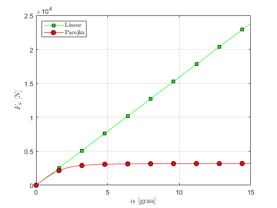
Tire model
Typical characteristic curve and slip angle definition

Pacejka
\[ F_{y} = D \sin \left[ C \arctan{B \alpha - E( B \alpha -\arctan(B \alpha))} \right] \]
Linear
\[ F_ y = K \alpha \]
clear ; close all ; clc

slipAngle = (0:0.1:15)*pi/180;         % Slip angle [rad]

% Pacejka tire parameters
a0  = 1;
a1  = 0;
a2  = 800;
a3  = 10000;
a4  = 50;
a5  = 0;
a6  = 0;
a7  = -1;
a8  = 0;
a9  = 0;
a10 = 0;
a11 = 0;
a12 = 0;
a13 = 0;

TirePac = VehicleDynamicsLateral.TirePacejka();

Fz          = 4e+03;
camber      = 0;
TirePac.a0  = a0;
TirePac.a1  = a1;
TirePac.a2  = a2;
TirePac.a3  = a3;
TirePac.a4  = a4;
TirePac.a5  = a5;
TirePac.a6  = a6;
TirePac.a7  = a7;
TirePac.a8  = a8;
TirePac.a9  = a9;
TirePac.a10 = a10;
TirePac.a11 = a11;
TirePac.a12 = a12;
TirePac.a13 = a13;

muy0    = TirePac.a1 * Fz/1000 + TirePac.a2;
D       = muy0 * Fz/1000;
BCD     = TirePac.a3 * sin(2 * atan(Fz/1000/TirePac.a4))*(1-TirePac.a5 * abs(camber));

% Pneu linear equivalente

Ktire   = BCD * 180/pi;

TireLin     = VehicleDynamicsLateral.TireLinear();
TireLin.k   = Ktire;

% Lateral force
FyPac = TirePac.Characteristic(slipAngle, Fz, muy0/1000);
FyLin = TireLin.Characteristic(slipAngle);

% Graphics
g = VehicleDynamicsLateral.Graphics(TirePac);
Comparison of tire models
figure(1)
ax = gca;
set(ax, 'NextPlot', 'add', 'Box', 'on', 'XGrid', 'on', 'YGrid', 'on')
p = plot(slipAngle * 180/pi,-FyLin, 'Color', 'g', 'Marker', 's', 'MarkerFaceColor', 'g', 'MarkeredgeColor', 'k', 'MarkerSize', 7);
g.changeMarker(p, 10);
p = plot(slipAngle * 180/pi,-FyPac, 'Color', 'r', 'Marker', 'o', 'MarkerFaceColor', 'r', 'MarkeredgeColor', 'k', 'MarkerSize', 7);
g.changeMarker(p, 10);
xlabel('\(\alpha\) [grau]', 'Interpreter', 'Latex')
ylabel('\(F_y\) [N]', 'Interpreter', 'Latex')
l = legend('Linear', 'Pacejka');
set(l, 'Interpreter', 'Latex', 'Location', 'NorthWest')

%
Plant model
Nonlinear vehicle + Pacejka tire
% Choosing vehicle
% System = VehicleDynamicsLateral.VehicleSimpleLinear();
VehiclePlant = VehicleDynamicsLateral.VehicleSimpleNonlinear();
% Defining vehicle parameters
VehiclePlant.mF0 = 700;
VehiclePlant.mR0 = 600;
VehiclePlant.IT = 10000;
VehiclePlant.lT = 3.5;
VehiclePlant.nF = 1;
VehiclePlant.nR = 1;
VehiclePlant.wT = 1.8;
VehiclePlant.muy = 1;
VehiclePlant.tire = TirePac;
VehiclePlant.deltaf = @ControlLaw;

disp(VehiclePlant)

% Choosing simulation
T       = 9;                     % Total simulation time             [s]
resol   = 500;                    % Resolution
TSPAN   = 0:T/resol:T;            % Time span                         [s]

simulator = VehicleDynamicsLateral.Simulator(VehiclePlant, TSPAN);
simulator.V0 = 16.7;
  VehicleSimpleNonlinear with properties:

        mT: 1300
        IT: 10000
         a: 1.6154
         b: 1.8846
       mF0: 700
       mR0: 600
        lT: 3.5000
        nF: 1
        nR: 1
        wT: 1.8000
       muy: 1
      tire: [1×1 VehicleDynamicsLateral.TirePacejka]
    deltaf: @ControlLaw
    deltar: 0
       Fxf: 0
       Fxr: 0
Controller design
Vehicle parameters
mT  = 1300;
IT  = 10000;
a   = 1.6154;
b   = 1.8846;
vT0 = 16.7;
KF  = Ktire;
KR  = Ktire;
Linear system
A = [      0   vT0            vT0                         0                       ;...
           0    0              0                          1                       ;...
           0    0      -(KF+KR)/(mT*vT0)  -(mT*vT0+(a*KF-b*KR)/(vT0))/(mT*vT0)    ;...
           0    0      -(a*KF-b*KR)/IT    -(a^2*KF+b^2*KR)/(IT*vT0)               ];

B = [   0                  ;...
        0                  ;...
        KF/(mT*vT0)        ;...
        a*KF/IT            ];


C = [1 0 0 0];
A
disp(A)
         0   16.7000   16.7000         0
         0         0         0    1.0000
         0         0   -8.3915   -0.9324
         0         0    2.4522   -3.3606
B
disp(B)
         0
         0
    4.1958
   14.7147
C
disp(C)
1 0 0 0
LQR design
Q = [   0.3 0 0 0 ;...
        0   1 0 0 ;...
        0   0 1 0 ;...
        0   0 0 1 ];
Q
disp(Q)

R = 1;
    0.3000         0         0         0
         0    1.0000         0         0
         0         0    1.0000         0
         0         0         0    1.0000
R
disp(R)

Klqr = lqr(A,B,Q,R);
1
Klqr
disp(Klqr)
0.5477 4.4651 1.0744 0.8169
Pole placement design
polos = [-6 -6.3 -6.7 -7];

Kplace = place(A,B,polos);
Kplace
disp(Kplace)
0.7936 6.6882 1.6107 0.5090
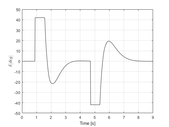
Control law
\[\delta = - {\bf K} {\bf z} + K_1 r \]
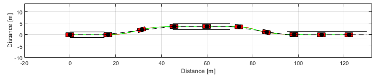
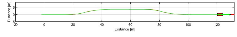
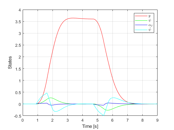
Double Lane Change Maneuver
% Simulation
simulator.Simulate();

g = VehicleDynamicsLateral.Graphics(simulator);
g.Frame();

    % Adding the double lane change track to the frame figure
    carWidth = 2;
    LaneOffset = 3.5;

    section1width = 1.1*carWidth + 0.25;
    section3width = 1.2*carWidth + 0.25;
    section5width = 1.3*carWidth + 0.25;

    section1Inf = -section1width/2;
    section1Sup = section1width/2;

    section3Inf = section1Inf+LaneOffset;
    section3Sup = section3Inf+section3width;
    section3Center = (section3Inf+section3Sup)/2;

    section5Inf = -section5width/2;
    section5Sup = section5width/2;

    % Section 1
    plot([0 15],[section1Inf section1Inf],'k')            % linha inferior
    plot([0 15],[section1Sup section1Sup],'k')            % linha superior
    plot([0 15],[0 0],'k--')                % linha central
    % Section 2
    plot([15 45],[0 section3Center],'k--')  % linha central
    % Section 3
    plot([45 70],[section3Inf section3Inf],'k')        % linha inferior
    plot([45 70],[section3Sup section3Sup],'k')        % linha superior
    plot([45 70],[section3Center section3Center],'k--')               % linha central
    % Section 4
    plot([70 95],[section3Center 0],'k--')
    % Section 5
    plot([95 130],[section5Inf section5Inf],'k')
    plot([95 130],[section5Sup section5Sup],'k')
    plot([95 130],[0 0],'k--')

g.Animation();
g.Animation();
% g.Animation('html/SteeringControlSimple');       % Uncomment to save animation gif

% Retrieving states
XT      = simulator.XT;
YT      = simulator.YT;
PSI     = simulator.PSI;
VEL     = simulator.VEL;
ALPHAT  = simulator.ALPHAT;
dPSI    = simulator.dPSI;

x = [YT PSI ALPHAT dPSI];

u = zeros(length(TSPAN),1);
output = zeros(length(TSPAN),1);

LateralDisp = 3.6;

for ii = 1:length(TSPAN)
    if XT(ii) <= 15
        r = 0;
    end
    if XT(ii) > 15 && XT(ii) <= 70
        r = LateralDisp;
    end
    if XT(ii) > 70
        r = 0;
    end

    u(ii) = - Kplace*x(ii,:)' + Kplace(1)*r;

    % Saturation
    if abs(u(ii)) < 42*pi/180
        output(ii) = u(ii);
    else
        output(ii) = sign(u(ii))*42*pi/180;
    end
end

% States
f = figure;
set(f,'PaperUnits','centimeters')
set(f,'PaperPosition',[0 0 8.9 5])
PaperPos = get(f,'PaperPosition');
set(f,'PaperSize',PaperPos(3:4))
hold on; box on; grid on
plot(TSPAN,YT,'r')
plot(TSPAN,PSI,'g')
plot(TSPAN,ALPHAT,'b')
plot(TSPAN,dPSI,'c')
xlabel('Time [s]')
ylabel('States')
l = legend('\(y\)','\(\psi\)','\(\alpha_T\)','\(\dot{\psi}\)');
set(l,'Interpreter','Latex','Location','NorthEast')

% Steering input
f = figure;
set(f,'PaperUnits','centimeters')
set(f,'PaperPosition',[0 0 8.9 3.5])
PaperPos = get(f,'PaperPosition');
set(f,'PaperSize',PaperPos(3:4))
hold on; box on; grid on
plot(TSPAN,output*180/pi,'k')
xlabel('Time [s]')
y = ylabel('\(\delta [deg]\)');
set(y,'Interpreter','Latex')