Kalman Filter - Simple vehicle

Kalman filter application for simple vehicle.

System
Plant
Maneuver
Modelo
Plant and model comparison
Model linearization
Medição
Verificação da linearização
Filtro estendido de Kalman
Comparação
Trajetória da estimativa
See Also

System

Consider a nonlinear stochastic vehicle model:

\[ \dot{{\bf x}} = {\bf f} ( {\bf x}(t) , t ) + {\bf G} (t) {\bf w} (t) \]

where

\({\bf w}\) white gaussian noise. \({\bf w}(t)\) ~ \(N ( {\bf 0} , {\bf Q}(t) )\)
\({\bf f} ( {\bf x}(t) , t )\) n-dimensional function \(n\)
\({\bf x}(t)\) state vector \((n \times 1)\)
\({\bf G}\) known matrix \((n \times s)\)

Plant

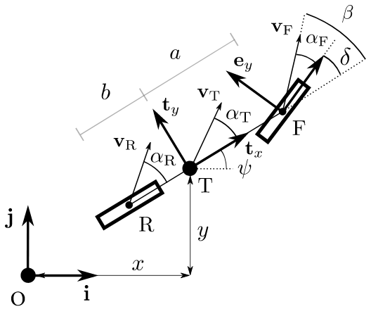
In this example, the plant is a nonlinear single track vehicle model with nonlinear tire model. See figure below

% Import the package with
%

import VehicleDynamicsLateral.*

Choosing tire and vehicle model.

TirePlant = TirePacejka;
disp(TirePlant)

VehiclePlant = VehicleSimpleNonlinear;
VehiclePlant.tire = TirePlant;
disp(VehiclePlant)

  TirePacejka with properties:

     a0: 1
     a1: 0
     a2: 800
     a3: 3000
     a4: 50
     a5: 0
     a6: 0
     a7: -1
     a8: 0
     a9: 0
    a10: 0
    a11: 0
    a12: 0
    a13: 0

  VehicleSimpleNonlinear with properties:

        mT: 1300
        IT: 10000
         a: 1.6154
         b: 1.8846
       mF0: 700
       mR0: 600
        lT: 3.5000
        nF: 2
        nR: 2
        wT: 2
       muy: 0.8000
      tire: [1×1 VehicleDynamicsLateral.TirePacejka]
    deltaf: 0
    deltar: 0
       Fxf: 0
       Fxr: 0

Maneuver

The maneuver to be estimated by the Kalman Filter is defined here.

Choosing simulation parameters:

T       = 6;                        % Total simulation time [s]
resol   = 50;                       % Resolution
TSPAN   = 0:T/resol:T;              % Time span             [s]

Running simulation.

simulatorPlant = Simulator(VehiclePlant, TSPAN);
simulatorPlant.dPSI0 = 0.35;
simulatorPlant.Simulate

Printing simulation parameters.

disp(simulatorPlant)

  Simulator with properties:

    Vehicle: [1×1 VehicleDynamicsLateral.VehicleSimpleNonlinear]
      TSpan: [51×1 double]
         X0: 0
         Y0: 0
       PSI0: 0
       PHI0: []
     THETA0: []
         V0: 20
    ALPHAT0: 0
      dPSI0: 0.3500
      dPHI0: []
    dTHETA0: []
         XT: [51×1 double]
         YT: [51×1 double]
        PSI: [51×1 double]
        PHI: []
      THETA: []
        VEL: [51×1 double]
     ALPHAT: [51×1 double]
       dPSI: [51×1 double]
       dPHI: []
     dTHETA: []

Retrieving states

XTPlant     = simulatorPlant.XT;
YTPlant     = simulatorPlant.YT;
PSIPlant    = simulatorPlant.PSI;
vTPlant     = simulatorPlant.VEL;
ALPHATPlant = simulatorPlant.ALPHAT;
dPSIPlant   = simulatorPlant.dPSI;

XOUTPlant   = [XTPlant YTPlant PSIPlant vTPlant ALPHATPlant dPSIPlant];

Generating graphics of the vehicle in the considered maneuver (plant)

gPlant = Graphics(simulatorPlant);
gPlant.TractorColor = 'r';
gPlant.Frame();

close all                   % Closing figures

Modelo

O modelo utilizado no algoritmo de estimação é baseado no mesmo modelo físico considerado no modelo da planta. Além disso, o modelo parte da premissa de que o projetista do estimador não tem conhecimento adequado da curva característica do pneu. Logo, o modelo de veículo é igual ao utilizado na planta, porém, o modelo de pneu é dado pelo modelo linear Tire linear, resultando num modelo do sistema de menor complexidade (em relação à planta) e com mais hipóteses simplificadoras.

Inicializando o pneu

TireModel = TireLinear;
disp(TireModel)

  TireLinear with properties:

    k: 40000

Choosing model vehicle

VehicleModel        = VehicleSimpleNonlinear; % Same as plant
VehicleModel.tire   = TireModel;
disp(VehicleModel)

  VehicleSimpleNonlinear with properties:

        mT: 1300
        IT: 10000
         a: 1.6154
         b: 1.8846
       mF0: 700
       mR0: 600
        lT: 3.5000
        nF: 2
        nR: 2
        wT: 2
       muy: 0.8000
      tire: [1×1 VehicleDynamicsLateral.TireLinear]
    deltaf: 0
    deltar: 0
       Fxf: 0
       Fxr: 0

Simulador com o mesmo vetor TSPAN e simulação

simulatorModel = Simulator(VehicleModel, TSPAN);
simulatorModel.dPSI0 = 0.35;
simulatorModel.Simulate;

disp(simulatorModel)

  Simulator with properties:

    Vehicle: [1×1 VehicleDynamicsLateral.VehicleSimpleNonlinear]
      TSpan: [51×1 double]
         X0: 0
         Y0: 0
       PSI0: 0
       PHI0: []
     THETA0: []
         V0: 20
    ALPHAT0: 0
      dPSI0: 0.3500
      dPHI0: []
    dTHETA0: []
         XT: [51×1 double]
         YT: [51×1 double]
        PSI: [51×1 double]
        PHI: []
      THETA: []
        VEL: [51×1 double]
     ALPHAT: [51×1 double]
       dPSI: [51×1 double]
       dPHI: []
     dTHETA: []

Retrieving states

XTModel = simulatorModel.XT;
YTModel = simulatorModel.YT;
PSIModel = simulatorModel.PSI;
vTModel = simulatorModel.VEL;
ALPHATModel = simulatorModel.ALPHAT;
dPSIModel = simulatorModel.dPSI;

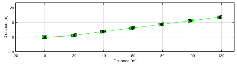
A manobra gerada pelo modelo escolhido pelo projetista a partir da mesma condição inicial é ilustrada na figura a seguir

gModel = Graphics(simulatorModel);
gModel.TractorColor = 'g';
gModel.Frame();

close all                   % Closing figures

Plant and model comparison

Comparando o modelo de pneu

g       = 9.81;
FzF     = VehiclePlant.mF0*g;
FzR     = VehiclePlant.mR0*g;
muy     = VehiclePlant.muy;
nF      = VehiclePlant.nF;
nR      = VehiclePlant.nR;

alpha   = 0:0.5:15;
alpha   = alpha*pi/180;
FyLin   = - TireModel.Characteristic(alpha);
FyFPac  = - TirePlant.Characteristic(alpha, FzF, muy);
FyRPac  = - TirePlant.Characteristic(alpha, FzR, muy);

figure
ax = gca;
set(ax,'NextPlot','add','Box','on','XGrid','on','YGrid','on')
plot(alpha(1:floor(end/2))*180/pi,FyLin(1:floor(end/2)),'r')
plot(alpha*180/pi,FyFPac,'g')
plot(alpha*180/pi,FyRPac,'g--')
xlabel('alpha [deg]')
ylabel('Fy [N]')
l = legend('Linear','Pacejka F','Pacejka R');
set(l,'Location','SouthEast')

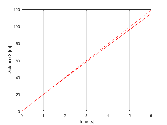
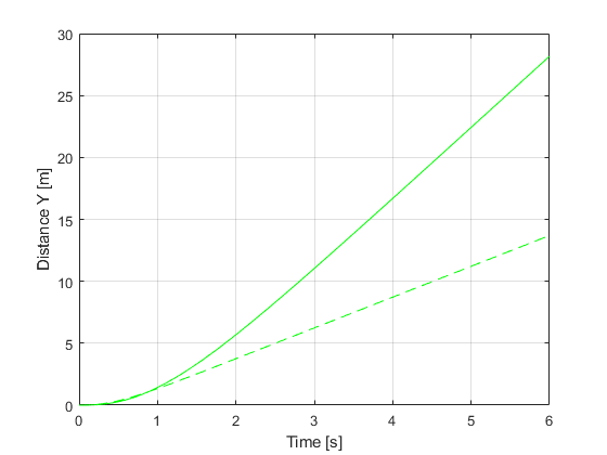
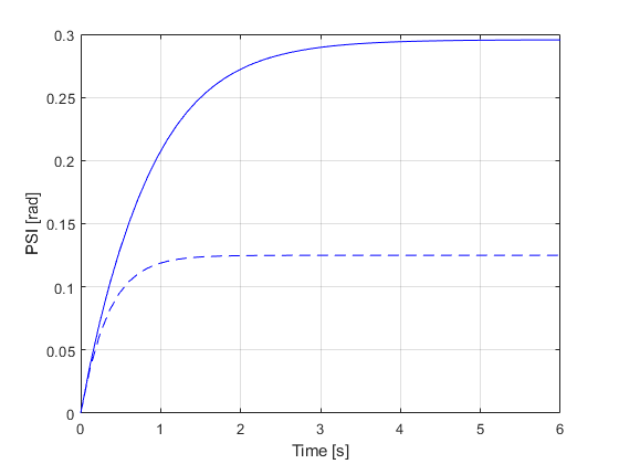
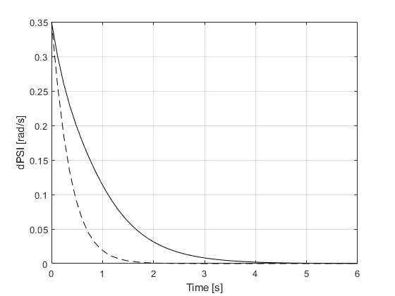
Comparando os estados

figure
ax = gca;
set(ax,'NextPlot','add','Box','on','XGrid','on','YGrid','on')
plot(TSPAN,XTPlant,'r')
plot(TSPAN,XTModel,'r--')
xlabel('Time [s]')
ylabel('Distance X [m]')

figure
ax = gca;
set(ax,'NextPlot','add','Box','on','XGrid','on','YGrid','on')
plot(TSPAN,YTPlant,'g')
plot(TSPAN,YTModel,'g--')
xlabel('Time [s]')
ylabel('Distance Y [m]')

figure
ax = gca;
set(ax,'NextPlot','add','Box','on','XGrid','on','YGrid','on')
plot(TSPAN,PSIPlant,'b')
plot(TSPAN,PSIModel,'b--')
xlabel('Time [s]')
ylabel('PSI [rad]')

figure
ax = gca;
set(ax,'NextPlot','add','Box','on','XGrid','on','YGrid','on')
plot(TSPAN,vTPlant,'c')
plot(TSPAN,vTModel,'c--')
xlabel('Time [s]')
ylabel('vT [m/s]')

figure
ax = gca;
set(ax,'NextPlot','add','Box','on','XGrid','on','YGrid','on')
plot(TSPAN,ALPHATPlant,'m'),
plot(TSPAN,ALPHATModel,'m--'),
xlabel('Time [s]')
ylabel('ALPHAT [rad/s]')

figure
ax = gca;
set(ax,'NextPlot','add','Box','on','XGrid','on','YGrid','on')
plot(TSPAN,dPSIPlant,'k')
plot(TSPAN,dPSIModel,'k--')
xlabel('Time [s]')
ylabel('dPSI [rad/s]')

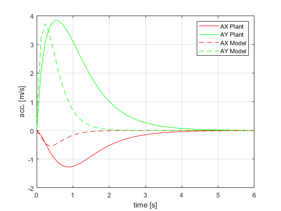
Comparando a aceleração longitudinal e transversal

saidasPlant = [XTPlant YTPlant PSIPlant vTPlant ALPHATPlant dPSIPlant];
matDerivEstadosPlant = zeros(size(saidasPlant));
for i = 1:size(saidasPlant,1)
    auxil = simulatorPlant.Vehicle.Model(1,saidasPlant(i,:),TSPAN);
    matDerivEstadosPlant(i,:) = auxil';
end

dXTPlant = matDerivEstadosPlant(:,1);
dYTPlant = matDerivEstadosPlant(:,2);
dPSIPlant = matDerivEstadosPlant(:,3);
dvTPlant = matDerivEstadosPlant(:,4);
dALPHATPlant = matDerivEstadosPlant(:,5);
ddPSIPlant = matDerivEstadosPlant(:,6);

ddXPlant = dvTPlant.*cos(PSIPlant + ALPHATPlant) - vTPlant.*(dPSIPlant + dALPHATPlant).*sin(PSIPlant + ALPHATPlant);
ddYPlant = dvTPlant.*sin(PSIPlant + ALPHATPlant) + vTPlant.*(dPSIPlant + dALPHATPlant).*cos(PSIPlant + ALPHATPlant);

ACELNumPlant = [(ddXPlant.*cos(PSIPlant) - ddYPlant.*sin(PSIPlant))  (-ddXPlant.*sin(PSIPlant) + ddYPlant.*cos(PSIPlant))];

saidasModel = [XTModel YTModel PSIModel vTModel ALPHATModel dPSIModel];
matDerivEstadosModel = zeros(size(saidasModel));
for i = 1:size(saidasModel,1)
    auxil = simulatorModel.Vehicle.Model(1,saidasModel(i,:),TSPAN);
    matDerivEstadosModel(i,:) = auxil';
end

dXTModel = matDerivEstadosModel(:,1);
dYTModel = matDerivEstadosModel(:,2);
dPSIModel = matDerivEstadosModel(:,3);
dvTModel = matDerivEstadosModel(:,4);
dALPHATModel = matDerivEstadosModel(:,5);
ddPSIModel = matDerivEstadosModel(:,6);

ddXModel = dvTModel.*cos(PSIModel + ALPHATModel) - vTModel.*(dPSIModel + dALPHATModel).*sin(PSIModel + ALPHATModel);
ddYModel = dvTModel.*sin(PSIModel + ALPHATModel) + vTModel.*(dPSIModel + dALPHATModel).*cos(PSIModel + ALPHATModel);

ACELNumModel = [(ddXModel.*cos(PSIModel) - ddYModel.*sin(PSIModel))  (-ddXModel.*sin(PSIModel) + ddYModel.*cos(PSIModel))];

figure
ax = gca;
set(ax,'NextPlot','add','Box','on','XGrid','on','YGrid','on')
plot(TSPAN,ACELNumPlant(:,1),'r')
plot(TSPAN,ACELNumPlant(:,2),'g')
plot(TSPAN,ACELNumModel(:,1),'r--')
plot(TSPAN,ACELNumModel(:,2),'g--')
xlabel('time [s]')
ylabel('acc. [m/s]')
l = legend('AX Plant','AY Plant','AX Model','AY Model');
set(l,'Location','NorthEast')

Comparando as derivadas dos estados

% figure
% ax = gca;
% set(ax,'NextPlot','add','Box','on','XGrid','on','YGrid','on')
% plot(TSPAN,dXTPlant,'r')
% plot(TSPAN,dXTModel,'r--')
% xlabel('Time [s]')
% ylabel('dX [m/s]')
% l = legend('Plant','Model');
% set(l,'Location','SouthWest')
%
% figure
% ax = gca;
% set(ax,'NextPlot','add','Box','on','XGrid','on','YGrid','on')
% plot(TSPAN,dYTPlant,'r')
% plot(TSPAN,dYTModel,'r--')
% xlabel('Time [s]')
% ylabel('dY [m/s]')
% l = legend('Plant','Model');
% set(l,'Location','NorthWest')
%
% figure
% ax = gca;
% set(ax,'NextPlot','add','Box','on','XGrid','on','YGrid','on')
% plot(TSPAN,dPSIPlant,'r')
% plot(TSPAN,dPSIModel,'r--')
% xlabel('Time [s]')
% ylabel('dPSI [rad/s]')
% l = legend('Plant','Model');
% set(l,'Location','NorthEast')
%
% figure
% ax = gca;
% set(ax,'NextPlot','add','Box','on','XGrid','on','YGrid','on')
% plot(TSPAN,dvTPlant,'r')
% plot(TSPAN,dvTModel,'r--')
% xlabel('Time [s]')
% ylabel('dvT [m/s]')
% l = legend('Plant','Model');
% set(l,'Location','SouthEast')
%
% figure
% ax = gca;
% set(ax,'NextPlot','add','Box','on','XGrid','on','YGrid','on')
% plot(TSPAN,dALPHATPlant,'r'),
% plot(TSPAN,dALPHATModel,'r--'),
% xlabel('Time [s]')
% ylabel('dALPHAT [rad/s]')
% l = legend('Plant','Model');
% set(l,'Location','NorthEast')
%
% figure
% ax = gca;
% set(ax,'NextPlot','add','Box','on','XGrid','on','YGrid','on')
% plot(TSPAN,ddPSIPlant,'r')
% plot(TSPAN,ddPSIModel,'r--')
% xlabel('Time [s]')
% ylabel('ddPSI [rad/s2]')
% l = legend('Plant','Model');
% set(l,'Location','SouthEast')

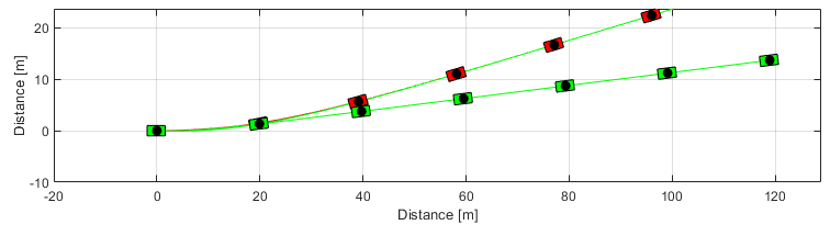
Comparação - Diferença de 10 m na direção X no momento da curva.

gModel.Frame();
hold on
gPlant.Frame();
gModel.Frame();

close all                   % Closing figures

Model linearization

A expressão geral da equação linearizada é obtida neste tópico utilizando o processador simbólico.

Definindo os símbolos:

syms XT YT PSI vT ALPHAT dPSI mT IT a b K

Slip angles

ALPHAF = atan((vT * sin(ALPHAT) + a * dPSI)/(vT * cos(ALPHAT))); % Dianteiro
ALPHAR = atan((vT * sin(ALPHAT) - b * dPSI)/(vT * cos(ALPHAT))); % Traseiro

pretty(ALPHAF)

    / a dPSI + vT sin(ALPHAT) \
atan| ----------------------- |
    \      vT cos(ALPHAT)     /

pretty(ALPHAR)

     / b dPSI - vT sin(ALPHAT) \
-atan| ----------------------- |
     \      vT cos(ALPHAT)     /

Lateral forces

FyF = -K*ALPHAF;
FyR = -K*ALPHAR;

pretty(FyF)

       / a dPSI + vT sin(ALPHAT) \
-K atan| ----------------------- |
       \      vT cos(ALPHAT)     /

pretty(FyR)

      / b dPSI - vT sin(ALPHAT) \
K atan| ----------------------- |
      \      vT cos(ALPHAT)     /

State equations

f1 = vT * cos(ALPHAT + PSI);
f2 = vT * sin(ALPHAT + PSI);
f3 = dPSI;
f4 = (FyF * sin(ALPHAT) + FyR * sin(ALPHAT))/(mT);
f5 = (FyF * cos(ALPHAT) + FyR * cos(ALPHAT) - mT * vT * dPSI) / (mT * vT);
f6 = (FyF * a - FyR * b) / IT;

f = [f1 ; f2 ; f3 ; f4 ; f5 ; f6];

pretty(f)

/                vT cos(ALPHAT + PSI)                \
|                                                    |
|                vT sin(ALPHAT + PSI)                |
|                                                    |
|                        dPSI                        |
|                                                    |
|          K #2 sin(ALPHAT) - K #1 sin(ALPHAT)       |
|        - -----------------------------------       |
|                           mT                       |
|                                                    |
|   dPSI mT vT + K cos(ALPHAT) #2 - K cos(ALPHAT) #1 |
| - ------------------------------------------------ |
|                         mT vT                      |
|                                                    |
|                    K a #2 + K b #1                 |
|                  - ---------------                 |
\                           IT                       /

where

             / b dPSI - vT sin(ALPHAT) \
   #1 == atan| ----------------------- |
             \      vT cos(ALPHAT)     /

             / a dPSI + vT sin(ALPHAT) \
   #2 == atan| ----------------------- |
             \      vT cos(ALPHAT)     /

Vetor de estados

States = [XT ; YT ; PSI ; vT ; ALPHAT ; dPSI];

pretty(States)

/   XT   \
|        |
|   YT   |
|        |
|   PSI  |
|        |
|   vT   |
|        |
| ALPHAT |
|        |
\  dPSI  /

O sistema linearizado é escrito na forma

\[ \dot{\bf x} = {\bf F} {\bf x} \]

onde \({\bf F}\) é a matriz dinâmica do modelo linear que é calculada a partir da equação não linear expandida em série de Taylor e truncada nos termos de primeira ordem. Logo, a matriz \({\bf F}\) é dada por

\[ {\bf F} = \left[ \frac{\partial f_i}{\partial x_j} \right]_{n \times n} \]

onde \(i\) e \(j\) indicam as equações e variÃ¡veis de estado utilizadas no cÃ¡lculo correpondente Ã posição \((i,j)\) da matriz jacobiana.

F = jacobian(f,States);
F = simplify(F);

pretty(F)

--
|
|
|
|  [0, 0, #6, cos(ALPHAT + PSI), #6, 0],
|
--

  [0, 0, #7, sin(ALPHAT + PSI), #7, 0], [0, 0, 0, 0, 0, 1],

  --
  |
  |                                    2       2      2     2
  |  0, 0, 0, -(K dPSI sin(2 ALPHAT) (a  b dPSI  - a b  dPSI
  --

                                     2       2
   + sin(ALPHAT) a b dPSI vT 4 - a vT  + b vT ))/(mT #2 #1 2),

         K vT sin(ALPHAT) #5   K vT sin(ALPHAT) #4
    #8 + ------------------- + -------------------
                  #2                    #1
  - ----------------------------------------------,
                          mT

    K a vT sin(2 ALPHAT)   K b vT sin(2 ALPHAT) --
    -------------------- - --------------------  |
            2 #2                   2 #1          |
  - -------------------------------------------  |,
                         mT                     --

  --
  |
  |             #8     K a dPSI #3   K b dPSI #3
  |  0, 0, 0, ------ - ----------- + -----------,
  |                2     mT vT #2      mT vT #1
  --          mT vT

    K vT cos(ALPHAT) #5                      K vT cos(ALPHAT) #4
    ------------------- - K sin(ALPHAT) #9 + -------------------
             #2                                       #1
  - ------------------------------------------------------------,
                                mT vT

            K a vT #3   K b vT #3 --
    mT vT - --------- + ---------  |
                #2          #1     |
  - -----------------------------  |,
                mT vT              |
                                  --

  --
  |
  |
  |                                   2  2     2                2
  |  0, 0, 0, (K dPSI cos(ALPHAT) (2 a  b  dPSI  - sin(ALPHAT) a  b dPSI vT
  --

        2   2                  2              2   2
   2 + a  vT  + sin(ALPHAT) a b  dPSI vT 2 + b  vT ))/(IT #2 #1),

                                2                     2                -- --
    K a vT #5   K b vT #4    K a  vT cos(ALPHAT)   K b  vT cos(ALPHAT)  |  |
    --------- - ---------    ------------------- + -------------------  |  |
        #2          #1                #2                    #1          |  |
  - ---------------------, - -----------------------------------------  |  |
              IT                                 IT                    --  |
                                                                          --

where

          2     2                               2
   #1 == b  dPSI  - sin(ALPHAT) b dPSI vT 2 + vT

          2     2                               2
   #2 == a  dPSI  + sin(ALPHAT) a dPSI vT 2 + vT

                    2
   #3 == sin(ALPHAT)  - 1

   #4 == vT - b dPSI sin(ALPHAT)

   #5 == vT + a dPSI sin(ALPHAT)

   #6 == -vT sin(ALPHAT + PSI)

   #7 == vT cos(ALPHAT + PSI)

   #8 == K cos(ALPHAT) #9

             / a dPSI + vT sin(ALPHAT) \       / b dPSI - vT sin(ALPHAT) \
   #9 == atan| ----------------------- | - atan| ----------------------- |
             \      vT cos(ALPHAT)     /       \      vT cos(ALPHAT)     /

Medição

Continuando simbolicamente, as grandezas medidas são:

Posição X
Posição Y
Aceleração angular
aceleração longitudinal
aceleração transversal

Para isso, utiliza-se as relações:

\[ \dot{x} = v_{\rm T} \cos \left( \psi + \alpha_{\rm T} \right) \]

\[ \dot{y} = v_{\rm T} \sin \left( \psi + \alpha_{\rm T} \right) \]

Aceleração

\[ \ddot{x} = \dot{v}_{\rm T} \cos \left( \psi + \alpha_{\rm T} \right) - v_{\rm T} \left( \dot{\psi} + \dot{\alpha}_{\rm T} \right) \sin \left( \psi + \alpha_{\rm T} \right) \]

\[ \ddot{y} = \dot{v}_{\rm T} \sin \left( \psi + \alpha_{\rm T} \right) + v_{\rm T} \left( \dot{\psi} + \dot{\alpha}_{\rm T} \right) \cos \left( \psi + \alpha_{\rm T} \right) \]

Implementando

ddX = f4*cos(PSI + ALPHAT) - vT*(dPSI + f5)*sin(PSI + ALPHAT);
ddY = f4*sin(PSI + ALPHAT) + vT*(dPSI + f5)*cos(PSI + ALPHAT);

Estes valores obtidos são as acelerações escritas na base fixa \(\{ O {\bf i} {\bf j} {\bf k} \}\). A projeção destas grandezas na base móvel \(\{ O {\bf t}_x {\bf t}_y {\bf t}_z \}\) é feita através da equação

\[ {\bf a} = \left( \ddot{x} \cos \psi - \ddot{y} \sin \psi \right) {\bf t}_x + \left( - \ddot{x} \sin \psi + \ddot{y} \sin \psi \right) {\bf t}_y \]

Implementando

ACEL = [ddX*cos(PSI) - ddY*sin(PSI) ; -ddX*sin(PSI) + ddY*cos(PSI)];
ACEL = simplify(ACEL);

pretty(ACEL)

/ K sin(2 PSI) #1 \
| --------------- |
|        mT       |
|                 |
|        K #1     |
|      - ----     |
\         mT      /

where

             / a dPSI + vT sin(ALPHAT) \       / b dPSI - vT sin(ALPHAT) \
   #1 == atan| ----------------------- | - atan| ----------------------- |
             \      vT cos(ALPHAT)     /       \      vT cos(ALPHAT)     /

A equação de observações não linear é dada por

\[ {\bf z}_k = {\bf h} ({\bf x}_k) + {\bf v}_k \]

com

\({\bf v}_k\) ~ \(N ( {\bf 0} , {\bf R}_k )\)

Linearizando termos

\[ {\bf z}_k = {\bf H} {\bf x}_k + {\bf v}_k \]

onde

\[ {\bf H} = \left[ \frac{\partial h_i}{\partial x_j} \right]_{m \times n} \]

ou seja, a matriz de saídas {\bf H} é a matriz jacobiana da equação de ACEL em relação aos estados.

Implementando

medNonlinear = [XT ; YT ; f6 ; ACEL];

H = jacobian(medNonlinear,States);
H = simplify(H);

pretty(H)

--
|
|
|
|  [1, 0, 0, 0, 0, 0], [0, 1, 0, 0, 0, 0],
--

  --
  |
  |
  |                                   2  2     2                2
  |  0, 0, 0, (K dPSI cos(ALPHAT) (2 a  b  dPSI  - sin(ALPHAT) a  b dPSI vT
  --

        2   2                  2              2   2
   2 + a  vT  + sin(ALPHAT) a b  dPSI vT 2 + b  vT ))/(IT #7 #6),

                                2                     2                --
    K a vT #5   K b vT #4    K a  vT cos(ALPHAT)   K b  vT cos(ALPHAT)  |
    --------- - ---------    ------------------- + -------------------  |
        #7          #6                #7                    #6          |
  - ---------------------, - -----------------------------------------  |,
              IT                                 IT                    --

  --
  |  0, 0,
  --

  /
  | K cos(2
  \

        /     / a dPSI + vT sin(ALPHAT) \
   PSI) | atan| ----------------------- |
        \     \      vT cos(ALPHAT)     /

         / b dPSI - vT sin(ALPHAT) \ \   \
   - atan| ----------------------- | | 2 |/mT,
         \      vT cos(ALPHAT)     / /   /

  K dPSI sin(2 PSI) cos(ALPHAT) #1  K sin(2 PSI) #2  K sin(2 PSI) #3 --
  --------------------------------, ---------------, ---------------  |,
              mT #7 #6                     mT               mT       --

                                                         --
                                                          |
                                                          |
  --            K dPSI cos(ALPHAT) #1    K #2    K #3 --  |
  |  0, 0, 0, - ---------------------, - ----, - ----  |  |
  --                   mT #7 #6           mT      mT  -- --

where

          2       2      2     2                                   2       2
   #1 == a  b dPSI  - a b  dPSI  + sin(ALPHAT) a b dPSI vT 4 - a vT  + b vT

         vT #5   vT #4
   #2 == ----- + -----
           #7      #6

         a vT cos(ALPHAT)   b vT cos(ALPHAT)
   #3 == ---------------- - ----------------
                #7                 #6

   #4 == vT - b dPSI sin(ALPHAT)

   #5 == vT + a dPSI sin(ALPHAT)

          2     2                               2
   #6 == b  dPSI  - sin(ALPHAT) b dPSI vT 2 + vT

          2     2                               2
   #7 == a  dPSI  + sin(ALPHAT) a dPSI vT 2 + vT

Verificação da linearização

Para verificar o procedimento de linearização, um ponto de operação referente Ã movimentação do veículo em linha reta com uma velocidade prescrita \(v_0\) é utilizado. Esta escolha é típica e pode ser verificada facilmente na literatura.

Definindo \(v_0\)

syms v0

Obtendo a matriz dinâmica

A = subs(F,States,[0 ; 0 ; 0 ; v0 ; 0 ; 0]);

pretty(A)

/ 0, 0,  0, 1,      0,               0          \
|                                               |
| 0, 0, v0, 0,      v0,              0          |
|                                               |
| 0, 0,  0, 0,      0,               1          |
|                                               |
| 0, 0,  0, 0,      0,               0          |
|                                               |
|                                     K a   K b |
|                             mT v0 + --- - --- |
|                   2 K                v0    v0 |
| 0, 0,  0, 0,   - -----,   - ----------------- |
|                  mT v0            mT v0       |
|                                               |
|                                   2      2    |
|                                K a    K b     |
|                                ---- + ----    |
|                K a - K b        v0     v0     |
| 0, 0,  0, 0, - ---------,    - -----------    |
\                    IT               IT        /

Obtendo a matriz de saídas

C = subs(H,States,[0 ; 0 ; 0 ; v0 ; 0 ; 0]);

pretty(C)

/ 1, 0, 0, 0,      0,             0        \
|                                          |
| 0, 1, 0, 0,      0,             0        |
|                                          |
|                                2      2  |
|                             K a    K b   |
|                             ---- + ----  |
|               K a - K b      v0     v0   |
| 0, 0, 0, 0, - ---------,  - -----------  |
|                   IT             IT      |
|                                          |
| 0, 0, 0, 0,      0,             0        |
|                                          |
|                              /  a    b \ |
|                            K | -- - -- | |
|                  2 K         \ v0   v0 / |
| 0, 0, 0, 0,    - ---,    - ------------- |
\                   mT             mT      /

Filtro estendido de Kalman

Implementação do algoritmo

Matriz que distribui o ruído na equação do estado constante

G = eye(6); % Matriz identidade (6 x 6)

Matrizes de covariância

Q = eye(6);
R = eye(5);

Matriz

P0 = eye(6);

Recuperando as condições iniciais usadas acima

X0Num = simulatorModel.X0;
Y0Num = simulatorModel.Y0;
PSI0Num = simulatorModel.PSI0;
VEL0Num = simulatorModel.V0;
ALPHAT0Num = simulatorModel.ALPHAT0;
dPSI0Num = simulatorModel.dPSI0;

x0 = [ X0Num ; Y0Num ; PSI0Num ; VEL0Num ; ALPHAT0Num ; dPSI0Num ];
x0 = zeros(6,1);
x0(4)=20;

Recuperando os parâmetros do veículo

mTNum = VehicleModel.mT;
ITNum = VehicleModel.IT;
aNum = VehicleModel.a;
bNum = VehicleModel.b;
KNum = TireModel.k;

parameters = [mTNum ITNum aNum bNum KNum];

Obtendo e verificando a aceleração que vai ser medida.

Inicializando o tempo de intervalo entre uma observação e outra.

intervalo = 0.1;

t = 0:intervalo:T;                  % Vetor com os instantes de observação

Prealocando

XOUTopt = zeros(length(t) + 1,length(States)); % Estimativa dos estados após atualização
Popt = zeros(length(t) + 1,1);                 % Matriz de covariância após atualização
Pantes = zeros(length(t) + 1,1);                 % Matriz de covariância antes da atualização
KKalmanopt = ones(length(t) + 1,1);                 % Ganho de Kalman

Atribuindo os primeiros valores

XOUTopt(1,:) = x0';
XOUTantes(1,:) = x0';
Pantes(1,1) = norm(P0);
Popt(1,1) = norm(P0);

% Distribuição dos erros

pesos = [5; 5; 0.1; 0.5; 0.5];

Iteração

for j = 1:length(t)
    % Ã?ndice variando por todos os instantes de observação

    % Vetor de tempo de integração para a etapa de propagação
    tspan = t(j):intervalo/100:t(j)+intervalo;

    % Obtendo as medidas da iteração
    z = [interp1(TSPAN,XTPlant(:,1),t(j)) ; interp1(TSPAN,YTPlant(:,1),t(j)) ; interp1(TSPAN,ddPSIPlant(:,1),t(j)) ; interp1(TSPAN,ACELNumPlant(:,1),t(j)) ; interp1(TSPAN,ACELNumPlant(:,2),t(j))];

    z = z + pesos.*(rand(5,1)-0.5);

    Fnum = subs(F,[States.' mT IT a b K],[x0.' parameters]);
    Fnum = double(Fnum);
    Hnum = subs(H,[States.' mT IT a b K],[x0.' parameters]);
    Hnum = double(Hnum);

    % Ciclo de propagação
    % Transformando a matriz PMat0 \((6 \times 6)\) em um vetor P0 \((1 \times 36)\)
    P0 = reshape(P0',[1 36]);

    [TOUT,Pout] = ode45(@(t,P) IntCov(t,P,Fnum,G,Q),tspan,P0);

    Pmatrix = reshape(Pout(end,:),[6 6])';

    simulatorKalman = Simulator(VehicleModel, tspan);
    % Definindo as condições iniciais
    simulatorKalman.X0 = x0(1);
    simulatorKalman.Y0 = x0(2);
    simulatorKalman.PSI0 = x0(3);
    simulatorKalman.V0 = x0(4);
    simulatorKalman.ALPHAT0 = x0(5);
    simulatorKalman.dPSI0 = x0(6);
    % Simulando
    simulatorKalman.Simulate()

    XTKalman = simulatorKalman.XT;
    YTKalman = simulatorKalman.YT;
    PSIKalman = simulatorKalman.PSI;
    vTKalman = simulatorKalman.VEL;
    ALPHATKalman = simulatorKalman.ALPHAT;
    dPSIKalman = simulatorKalman.dPSI;

    XOUTKalman = [XTKalman YTKalman PSIKalman vTKalman ALPHATKalman dPSIKalman];

    % Ciclo de atualização

    ACELKalman = subs(medNonlinear,[States.' mT IT a b K],[XOUTKalman(end,:) parameters]);
    ACELKalman = double(ACELKalman);

    KKalman = Pmatrix*Hnum' / (Hnum*Pmatrix*Hnum' + R);

    XKalman = XOUTKalman(end,:)' + KKalman*(z - ACELKalman);
    PKalman = Pmatrix - KKalman*Hnum*Pmatrix;

    x0 = XKalman;
    P0 = PKalman;

    XOUTopt(j+1,:) = XKalman';
    XOUTantes(j+1,:) = XOUTKalman(end,:);
    Popt(j+1) = norm(PKalman);
    Pantes(j+1) = norm(Pmatrix);
    KKalmanopt(j+1) = norm(KKalman);

end

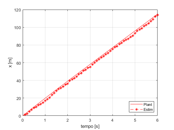
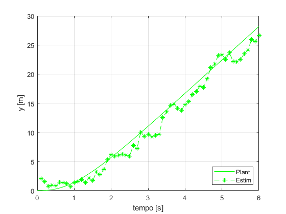
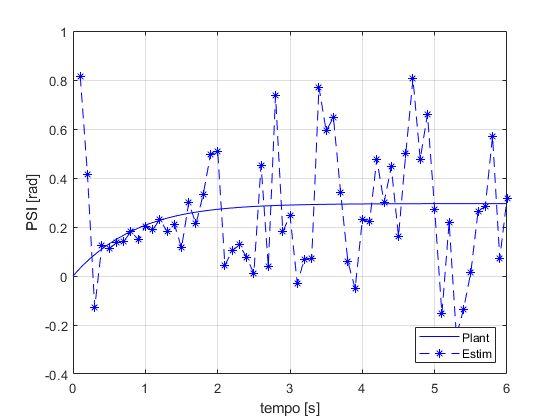
Comparação

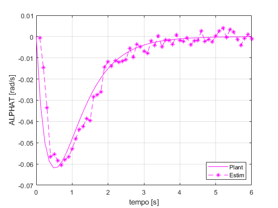
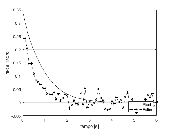
figure
ax = gca;
set(ax,'NextPlot','add','Box','on','XGrid','on','YGrid','on')
plot(TSPAN,XOUTPlant(:,1),'r')
p = plot(t(2:end),XOUTopt(2:end-1,1),'r--');
set(p,'Marker','*')
l = legend('Plant','Estim');
set(l,'Location','SouthEast')
xlabel('tempo [s]')
ylabel('x [m]')

figure
ax = gca;
set(ax,'NextPlot','add','Box','on','XGrid','on','YGrid','on')
plot(TSPAN,XOUTPlant(:,2),'g')
p = plot(t(2:end),XOUTopt(2:end-1,2),'g--');
set(p,'Marker','*')
l = legend('Plant','Estim');
set(l,'Location','SouthEast')
xlabel('tempo [s]')
ylabel('y [m]')

figure
ax = gca;
set(ax,'NextPlot','add','Box','on','XGrid','on','YGrid','on')
plot(TSPAN,XOUTPlant(:,3),'b')
p = plot(t(2:end),XOUTopt(2:end-1,3),'b--');
set(p,'Marker','*')
l = legend('Plant','Estim');
set(l,'Location','SouthEast')
xlabel('tempo [s]')
ylabel('PSI [rad]')

figure
ax = gca;
set(ax,'NextPlot','add','Box','on','XGrid','on','YGrid','on')
plot(TSPAN,XOUTPlant(:,4),'c')
p = plot(t(2:end),XOUTopt(2:end-1,4),'c--');
set(p,'Marker','*')
l = legend('Plant','Estim');
set(l,'Location','SouthEast')
xlabel('tempo [s]')
ylabel('vT [m/s]')

figure
ax = gca;
set(ax,'NextPlot','add','Box','on','XGrid','on','YGrid','on')
plot(TSPAN,XOUTPlant(:,5),'m')
p = plot(t(2:end),XOUTopt(2:end-1,5),'m--');
set(p,'Marker','*')
l = legend('Plant','Estim');
set(l,'Location','SouthEast')
xlabel('tempo [s]')
ylabel('ALPHAT [rad/s]')

figure
ax = gca;
set(ax,'NextPlot','add','Box','on','XGrid','on','YGrid','on')
plot(TSPAN,XOUTPlant(:,6),'k')
p = plot(t(2:end),XOUTopt(2:end-1,6),'k--');
set(p,'Marker','*')
l = legend('Plant','Estim');
set(l,'Location','SouthEast')
xlabel('tempo [s]')
ylabel('dPSI [rad/s]')

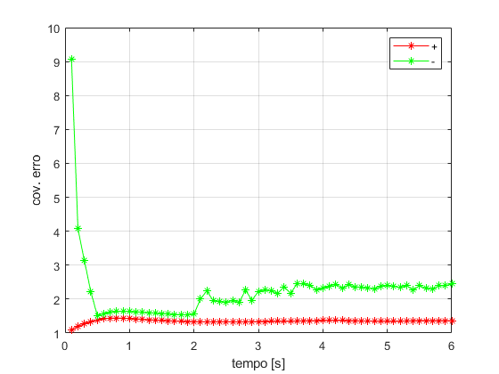
Cov. do erro

figure
ax = gca;
set(ax,'NextPlot','add','Box','on','XGrid','on','YGrid','on')
p = plot(t(2:end),KKalmanopt(2:end-1),'r');
set(p,'Marker','*')
ylabel('ganho de kalman')
xlabel('tempo [s]')

figure
ax = gca;
set(ax,'NextPlot','add','Box','on','XGrid','on','YGrid','on')
p = plot(t(2:end),Popt(2:end-1),'r');
set(p,'Marker','*')
p = plot(t(2:end),Pantes(2:end-1),'g');
set(p,'Marker','*')
l = legend('+','-');
set(l,'Location','NorthEast')
ylabel('cov. erro')
xlabel('tempo [s]')

close all

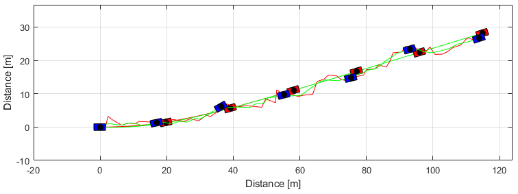
Trajetória da estimativa

Usando o simulatorPlant para inicializar o Graphics do Kalman

gKalman = Graphics(simulatorKalman);
gKalman.Simulator.TSpan     = t;
gKalman.Simulator.XT        = XOUTopt(1:end-1,1);
gKalman.Simulator.YT        = XOUTopt(1:end-1,2);
gKalman.Simulator.PSI       = XOUTopt(1:end-1,3);
gKalman.Simulator.VEL       = XOUTopt(1:end-1,4);
gKalman.Simulator.ALPHAT    = XOUTopt(1:end-1,5);
gKalman.Simulator.dPSI      = XOUTopt(1:end-1,6);
gKalman.TractorColor        = 'b';
gKalman.Frame()

close all

gPlant.Frame();
hold on
% gModel.Frame();
gKalman.Frame();

Kalman Filter - Simple vehicle

Contents

System

Plant

Maneuver

Modelo

Plant and model comparison

Model linearization

Medição

Verificação da linearização

Filtro estendido de Kalman

Comparação

Trajetória da estimativa

See Also